I Taught My Phone to Know I'm Lying on the Couch. Here's How.

I’ve been fascinated by real-time signal processing for a while. You know that feeling when you’re watching a live graph of sensor data and it wiggles around in response to the real world? That’s basically digital sorcery and I love it.

I was thinking where to get the data and what to classify.

One day I thought: what if I could make my phone figure out what I’m doing, just from its motion sensors?

Simple idea. Should be easy enough for 2 days of tinkering, right?

What We’re Building Link to heading

Human Activity Recognition (HAR) — the phone watches how you’re moving and says “ah yes, you are walking” or “you are definitely just standing in the kitchen pretending you’re about to be productive.”

We’ll classify three activities:

Standing (doing nothing, full of potential)
Walking (going somewhere, probably the fridge)
Jumping (because science needs suffering)

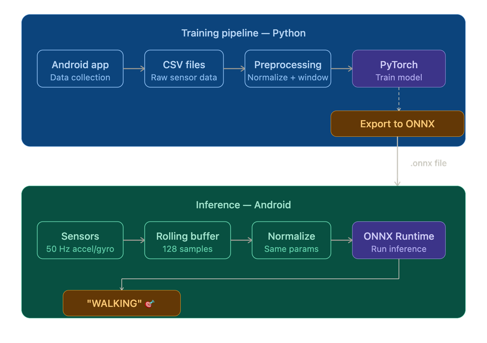
The full pipeline looks like this:

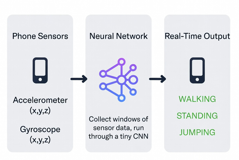
Let’s go step by step.

Step 1: The Data — Become a Human Tripod Link to heading

Before we can train anything, we need labeled sensor data. I built a simple Android app that records accelerometer and gyroscope readings at 50Hz (50 samples per second) and lets me tag what activity I’m doing.

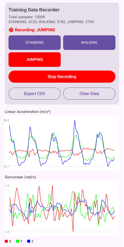
Step 1: The Data — Become a Human Tripod Link to heading

Why 50Hz specifically? Link to heading

Human movement is slow by physics standards. A walking step takes around 0.5–1 second, a jump maybe 0.3–0.5 seconds. To reliably capture those shapes in sensor data, you need to sample at least twice as fast as the fastest thing you’re trying to see — that’s the Nyquist theorem doing its thing. 50Hz is overkill for walking and just right for jumping. 10Hz would turn your jump into a vague blip. 200Hz would just be redundant data burning battery.

Why both accelerometer and gyroscope? Link to heading

The accelerometer tells you about linear forces — how hard the phone is being pushed in any direction. The gyroscope tells you about rotation. Standing still, both are quiet. Walking gives you periodic acceleration spikes as each foot lands. Jumping gives you a brief moment of near-weightlessness (free-fall), a huge spike on landing, and a lot of rotation if you’re anything like me. Together they’re more informative than either alone.

From the two sensors we get 6 raw features (x, y, z for each). I added two more derived ones to give the network a little head start:

Feature	What it is	Why it helps
acc_x, acc_y, acc_z	Accelerometer axes (m/s²)	Raw motion
gyro_x, gyro_y, gyro_z	Gyroscope axes (rad/s)	Rotation
acc_mag_sq	acc_x² + acc_y² + acc_z²	“How much am I moving, total?”
gyro_mag_sq	gyro_x² + gyro_y² + gyro_z²	“How much am I spinning, total?”

Why those two derived features? Because they’re orientation-independent. If you carry your phone in your pocket, your right pocket, your hand, your left hand — the individual x/y/z values change completely depending on how the phone is rotated. But the magnitude — the total force vector, regardless of direction — stays consistent.

So 8 features per sample.

I spent ~15 minutes being a test subject for my own app:

5 minutes walking around my apartment like a Roomba
5 minutes standing perfectly still, contemplating my life choices
5 minutes jumping — my downstairs neighbor is filing paperwork as we speak

Result: ~15,000 samples per activity. Small dataset. Enough to prove a point.

Step 2: Preprocessing — Making the Data Neural-Network-Friendly Link to heading

Raw sensor numbers go from roughly -20 to +20 for accelerometer, and -10 to +10 for gyroscope. Neural networks are picky eaters — they work best when all the data is in a similar, nice range.

Z-Score Normalization Link to heading

We subtract the mean and divide by the standard deviation for each feature. Think of it as “making everyone the same height before a team photo.”

The formula:

x_normalized = (x - mean) / std_deviation

Why does this matter? Neural networks learn by adjusting weights based on gradients — essentially, tiny nudges in the right direction. If one feature has values in the thousands and another in the hundredths, the gradients end up wildly different in scale.

Important: we compute the mean and std from the training data only, then save those values. The Android app will need them later to normalize incoming sensor data before feeding it to the model.

Windowing — Turning a Stream into Chunks Link to heading

The network doesn’t look at individual samples. It looks at windows — a batch of 128 consecutive samples fed in at once.

Why not just classify sample by sample? A single accelerometer reading tells you almost nothing. At any given instant, standing still and the top of a jump can produce nearly identical values — both involve near-zero acceleration. What distinguishes them is the shape over time: the pattern of readings before and after. A window gives the model enough temporal context to actually make a decision.

At 50Hz, 128 samples = ~2.56 seconds of movement. Here’s the idea:

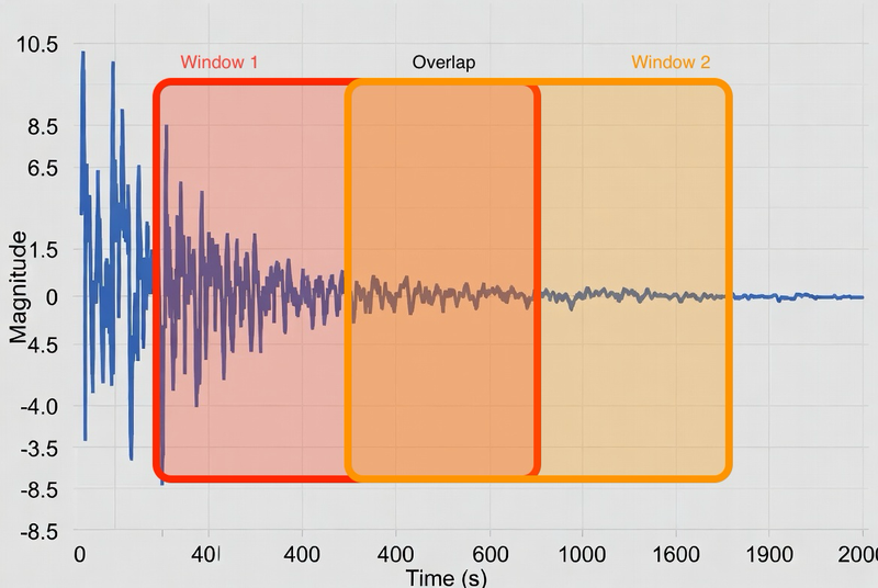
Why 50% overlap? Two reasons. First, activity transitions — if you go from standing to walking mid-window, a non-overlapping scheme might produce a window that’s half standing / half walking and gets mislabeled. Second, overlap is free data augmentation.

Each window gets a single label based on majority vote of what the samples inside it were labeled as.

70% goes to training, 15% to validation, 15% to testing. Don’t mix future data into training — that’s called data leakage and it’s the machine learning equivalent of open-book cheating.

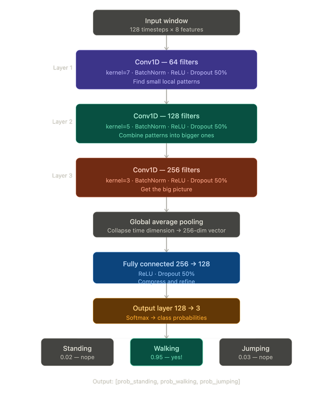
Step 3: The Neural Network — The Actual Scary Part Link to heading

If you’re an Android dev reading this going “what is a neural network” — don’t panic. Here’s the one-paragraph version.

A neural network is a function with a lot of tunable parameters (called weights). You show it thousands of labeled examples, it makes wrong guesses, you tell it how wrong it was, and it nudges its weights to be slightly less wrong next time. Do that enough times and it starts getting things right. That’s machine learning.

For this project I used a 1D Convolutional Neural Network (CNN). The “1D” part means it slides a filter along one dimension — in our case, time. It’s really good at spotting repeating patterns in sequences: “oh, this wiggly shape in the accelerometer every 0.5 seconds? That’s a walking step.”

Here’s the architecture:

Why a CNN and not something else? Link to heading

You might have heard of other architectures — LSTMs, Transformers, plain dense networks. CNNs are a good fit here for a few reasons. Dense networks would treat every timestep independently, with no notion of things happening next to each other in time. LSTMs are good at long-range dependencies but slower to train and harder to export to mobile. Transformers are powerful but massively overkill for 2.56 seconds of motion data — they’d be like hiring a symphony orchestra to play a ringtone.

The whole model has about 243,000 parameters. That sounds like a lot but it’s tiny by modern standards — it’s under 1MB and runs comfortably on a phone.

Annotations Link to heading

BatchNorm — normalizes the data between layers so training is stable. Think of it as a shock absorber.
ReLU — the activation function. It just returns max(0, x). Without a non-linear activation function between layers, stacking layers would be mathematically equivalent to having a single layer.
Dropout — randomly zeroes out 50% of neurons during training. Forces the network to not rely too heavily on any one path.
Global Average Pooling — takes the 128-timestep output and collapses it to a single number per filter.

Step 4: Training — Watching Numbers Go Down Link to heading

Training is the part where the network actually learns. We:

Feed it a batch of windows
It makes predictions (badly, at first)
We measure how wrong it was (the loss)
We nudge all the weights slightly in the direction that reduces the loss (backpropagation)
Repeat ~5000 times

Settings I used:

Loss function: Cross-Entropy Loss — standard for “pick one of N classes” problems
Optimizer: Adam — a smarter version of gradient descent
Learning rate: 0.001
Batch size: 32
Early stopping: if validation accuracy doesn’t improve for 15 epochs, we stop
Device: MPS (Apple Silicon GPU) — because waiting is suffering

The training runs for maybe 50–80 epochs before early stopping kicks in. Takes a few minutes on a laptop.

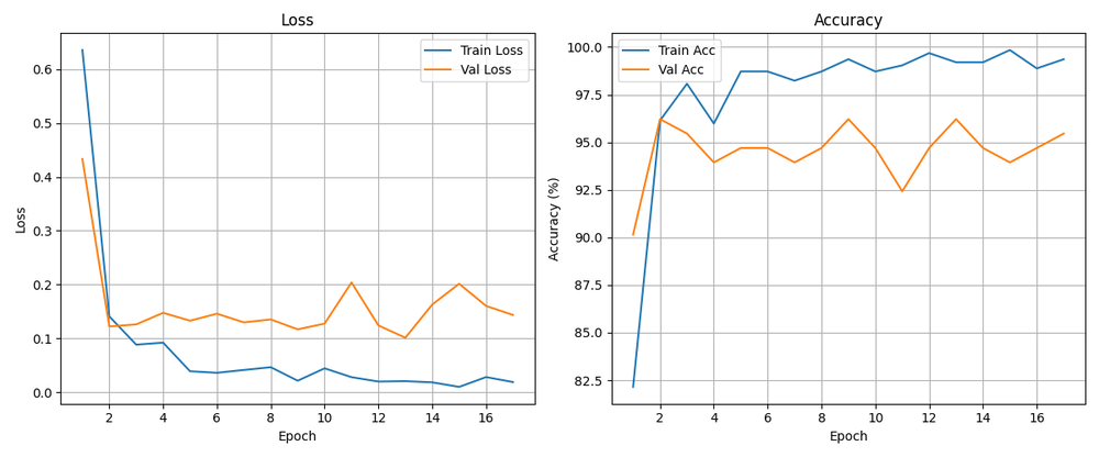
Step 5: Evaluation — Did It Actually Learn Anything? Link to heading

Time to test it on data it’s never seen.

Test Accuracy: 97.73% 

              precision  recall  f1-score
STANDING          0.98      1.00     0.99
WALKING           0.97      0.99     0.98
JUMPING           1.00      0.82     0.90

Confusion Matrix:
              STANDING  WALKING  JUMPING
STANDING          48        0       0
WALKING            1       72       0
JUMPING            0        2       9

97.73%. Not bad for a model trained on one person walking around their apartment for 15 minutes.

What do precision and recall actually mean? For Android devs: think of precision as “when the model says X, how often is it right?” and recall as “out of all the actual X cases, how many did the model catch?”

Reading the confusion matrix:

Standing: perfect. Never confused with anything.
Walking: one sample got mistaken for standing. One. Probably the moment I paused to check my phone.
Jumping: 2 jumps were classified as walking. Honestly, near the end of the recording session I was jumping pretty half-heartedly. Can’t blame the model.

Step 6: Running It on Android — A Brief Tour of Model Formats Link to heading

Every ML project has a moment where the model works great in Python and you think “okay, how hard can it be to run this on a phone?” The answer is: not that hard, you just have to pick the right format on the first try. I did not pick the right format on the first try.

Attempt 1: PyTorch Mobile Link to heading

PyTorch has an official mobile library. Added the dependency, hit Run, got this:

UnsatisfiedLinkError: dlopen failed: 
"libtorch_android_pytorch_jni.so" has unexpected page size

PyTorch Mobile doesn’t support 16KB page sizes, which modern Android requires. Cool cool cool. Next.

Attempt 2: TensorFlow Lite Link to heading

TFLite is the established standard for ML on Android. The docs mention, casually, that it requires a Linux environment. I’m on a Mac. We move on without making eye contact.

Attempt 3: ONNX — This One Actually Works Link to heading

ONNX (Open Neural Network Exchange) is an open model format that works across frameworks and platforms. Android supports it via ONNX Runtime, which also supports NNAPI hardware acceleration on Android.

Why does ONNX work where the others didn’t? ONNX was designed from the start to be a transport format — platform-agnostic, just a standardized description of your computation graph.

Converting the model is surprisingly painless:

dummy_input = torch.randn(1, 128, 8)  # fake input to trace the model's shape

torch.onnx.export(
    model,
    dummy_input,
    "har_model.onnx",
    input_names=["input"],
    output_names=["output"],
    dynamic_axes={"input": {0: "batch"}, "output": {0: "batch"}},
    opset_version=17,
)

This produces a har_model.onnx file that’s about 1MB.

Android Integration Link to heading

Three files go into app/src/main/assets/:

har_model.onnx — the trained model (~1MB)
har_model.onnx.data — model weights data
normalization_params.json — mean + std for each of 8 features

The inference loop in Kotlin is straightforward with ONNX Runtime.

Why a circular/rolling buffer? In training we had a static CSV we could slice up at will. On the phone, sensor data arrives continuously, one sample at a time. The circular buffer is the bridge between “event-driven stream” and “fixed-size window” — it holds the last 128 samples at all times.

The Full Picture Link to heading

Let’s zoom out:

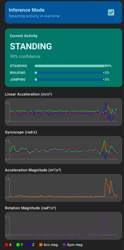
And the final Android demo:

What I Learned Link to heading

Machine learning turned out to be less mysterious than I expected. Training a model is basically: show it examples, tell it when it’s wrong, let it adjust. The parts that actually require attention are the decisions around the model — how you collect data, how you preprocess it, and how faithfully you reproduce that preprocessing at inference time.

ML on Android — the model format situation is a bit of a maze, but once you find the right door (ONNX), it’s genuinely smooth. Just go straight to ONNX.

The real lesson: the machine learning part is often the easy part. A 98% accurate model trained in an afternoon, on data collected by jumping around an apartment. The hard part is the pipeline around it — getting data to flow cleanly from raw sensor readings all the way to a real-time prediction without anything silently breaking in the middle. That’s just software engineering. And you already know how to do that.

Source Code Link to heading

The complete code — Python training scripts + Android app — is available in the repository.

Repository: https://github.com/eziosoft/ActivityClassifierDemo_Android

If your phone now knows you’re just standing in the kitchen pretending to be productive, I’m sorry. I built this.